Gaining insights on Wine quality from its constituents
Synopsis
The Goal of this project is to apply statistical learning methods to answer the following interesting questions:
- Which constituents(predictors) found in wine are associated with the wine quality(response)
- Understanding the relationship between the response and predictors
Relevant information: The data is obtained from the source UCI ML datbase.The data was compiled from results of chemical analyses of wines grown in same region in Italy using different cultivars. The dataset has 1599 observation with 12 variables and “quality” is the interested response.
Overview of Analysis approach
- Data Pre-processing
- Forward step-wise selection
- Model-selection using K-fold cross validation
- Inferences from the best-final model
Data pre-processing
The data is loaded as wine, and the response variable is plotted. Then we examine the predictor variables and observations containing “NA” values are omitted. The data is then split into Train and Test dataset. The Train dataset is used for learning the parameters related to the model and the test data is used for final evaluation.
library(readr)
library(knitr)
wine <- read_delim("F:/subhash/UCI datasets/regerssion/Wine quality/winequality-red.csv",
    ";", escape_double = FALSE, trim_ws = TRUE)
kable(head(wine),caption = "Wine dataframe")
| fixed acidity | volatile acidity | citric acid | residual sugar | chlorides | free sulfur dioxide | total sulfur dioxide | density | pH | sulphates | alcohol | quality |
|---|---|---|---|---|---|---|---|---|---|---|---|
| 7.4 | 0.70 | 0.00 | 1.9 | 0.076 | 11 | 34 | 0.9978 | 3.51 | 0.56 | 9.4 | 5 |
| 7.8 | 0.88 | 0.00 | 2.6 | 0.098 | 25 | 67 | 0.9968 | 3.20 | 0.68 | 9.8 | 5 |
| 7.8 | 0.76 | 0.04 | 2.3 | 0.092 | 15 | 54 | 0.9970 | 3.26 | 0.65 | 9.8 | 5 |
| 11.2 | 0.28 | 0.56 | 1.9 | 0.075 | 17 | 60 | 0.9980 | 3.16 | 0.58 | 9.8 | 6 |
| 7.4 | 0.70 | 0.00 | 1.9 | 0.076 | 11 | 34 | 0.9978 | 3.51 | 0.56 | 9.4 | 5 |
| 7.4 | 0.66 | 0.00 | 1.8 | 0.075 | 13 | 40 | 0.9978 | 3.51 | 0.56 | 9.4 | 5 |
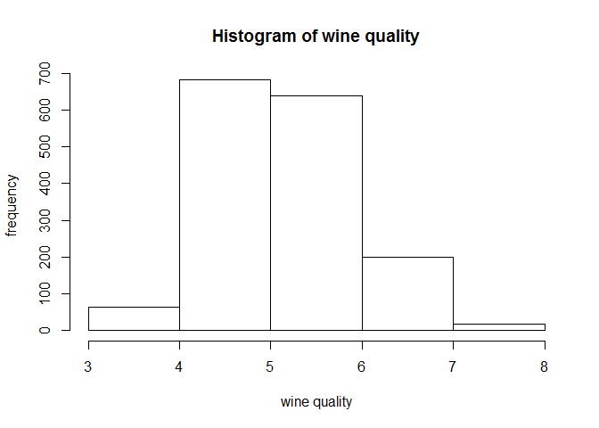
hist(wine$quality,breaks =5,xlab="wine quality",ylab = "frequency",main = "Histogram of wine quality")
fivenum(wine$quality)
## [1] 3 5 6 6 8
It is noted that the wine quality has a normal distribution(approx.) and the minimum and maximum values are 3 and 8 respectively, wit median at 6.Next we look at summary of our data to find are there any NA/missing values.
summary(wine)
##  fixed acidity   volatile acidity  citric acid    residual sugar
##  Min.   : 4.60   Min.   :0.1200   Min.   :0.000   Min.   : 0.900
##  1st Qu.: 7.10   1st Qu.:0.3900   1st Qu.:0.090   1st Qu.: 1.900
##  Median : 7.90   Median :0.5200   Median :0.260   Median : 2.200
##  Mean   : 8.32   Mean   :0.5278   Mean   :0.271   Mean   : 2.539
##  3rd Qu.: 9.20   3rd Qu.:0.6400   3rd Qu.:0.420   3rd Qu.: 2.600
##  Max.   :15.90   Max.   :1.5800   Max.   :1.000   Max.   :15.500
##
##    chlorides       free sulfur dioxide total sulfur dioxide
##  Min.   :0.01200   Min.   : 1.00       Min.   :  6.00
##  1st Qu.:0.07000   1st Qu.: 7.00       1st Qu.: 22.00
##  Median :0.07900   Median :14.00       Median : 38.00
##  Mean   :0.08747   Mean   :15.87       Mean   : 46.43
##  3rd Qu.:0.09000   3rd Qu.:21.00       3rd Qu.: 62.00
##  Max.   :0.61100   Max.   :72.00       Max.   :289.00
##                                        NA's   :2
##     density             pH          sulphates         alcohol
##  Min.   :0.9901   Min.   :2.740   Min.   :0.3300   Min.   : 8.40
##  1st Qu.:0.9956   1st Qu.:3.210   1st Qu.:0.5500   1st Qu.: 9.50
##  Median :0.9968   Median :3.310   Median :0.6200   Median :10.20
##  Mean   :0.9967   Mean   :3.311   Mean   :0.6581   Mean   :10.42
##  3rd Qu.:0.9978   3rd Qu.:3.400   3rd Qu.:0.7300   3rd Qu.:11.10
##  Max.   :1.0037   Max.   :4.010   Max.   :2.0000   Max.   :14.90
##
##     quality
##  Min.   :3.000
##  1st Qu.:5.000
##  Median :6.000
##  Mean   :5.636
##  3rd Qu.:6.000
##  Max.   :8.000
##
We see there are 2 NA values in the “total sulphur dioxide” variable, this missing values are handled by removing the observations corresponding to it. We’ll also look the description of the variables(understood from the var names)and their type
| Attribute | variable type |
|---|---|
| Fixed Acidity | Continuous |
| Volatile Acidity | Continuous |
| Citric acid | Continuous |
| Residual sugar | Continuous |
| Chlorides | Continuous |
| free sulfur dioxide | Continuous |
| total sulfur dioxide | Continuous |
| density | Continuous |
| pH | Continuous |
| sulphates | Continuous |
| alcohol | Continuous |
| quality | Continuous |
wine<-na.omit(wine)
set.seed(1)
ind=sample(seq(1597),1280,replace=FALSE)
wine_train<-wine[ind,]
wine_test<-wine[-ind,]
Linear model selection
Here we use forward stepwise selection, a computationally efficient method to find the best set of predictors related to the response variable. Brief overview: It begins with a model containing no predictors, and then adds predictors to the model one at a time, until all predictors are in the model. At each step we have p − k models where p refers to total number of predictors and k represents the step index. We have approximately p2 models which is further reduced to p models.
library(leaps)
regfit.fwd=regsubsets(quality~.,data=wine_train,nvmax=11,method="forward")
summary(regfit.fwd)
## Subset selection object
## Call: regsubsets.formula(quality ~ ., data = wine_train, nvmax = 11,
##     method = "forward")
## 11 Variables  (and intercept)
##                        Forced in Forced out
## `fixed acidity`            FALSE      FALSE
## `volatile acidity`         FALSE      FALSE
## `citric acid`              FALSE      FALSE
## `residual sugar`           FALSE      FALSE
## chlorides                  FALSE      FALSE
## `free sulfur dioxide`      FALSE      FALSE
## `total sulfur dioxide`     FALSE      FALSE
## density                    FALSE      FALSE
## pH                         FALSE      FALSE
## sulphates                  FALSE      FALSE
## alcohol                    FALSE      FALSE
## 1 subsets of each size up to 11
## Selection Algorithm: forward
##           `fixed acidity` `volatile acidity` `citric acid`
## 1  ( 1 )  " "             " "                " "
## 2  ( 1 )  " "             "*"                " "
## 3  ( 1 )  " "             "*"                " "
## 4  ( 1 )  " "             "*"                " "
## 5  ( 1 )  " "             "*"                " "
## 6  ( 1 )  " "             "*"                " "
## 7  ( 1 )  " "             "*"                " "
## 8  ( 1 )  " "             "*"                " "
## 9  ( 1 )  " "             "*"                "*"
## 10  ( 1 ) "*"             "*"                "*"
## 11  ( 1 ) "*"             "*"                "*"
##           `residual sugar` chlorides `free sulfur dioxide`
## 1  ( 1 )  " "              " "       " "
## 2  ( 1 )  " "              " "       " "
## 3  ( 1 )  " "              " "       " "
## 4  ( 1 )  " "              "*"       " "
## 5  ( 1 )  " "              "*"       " "
## 6  ( 1 )  " "              "*"       " "
## 7  ( 1 )  " "              "*"       "*"
## 8  ( 1 )  "*"              "*"       "*"
## 9  ( 1 )  "*"              "*"       "*"
## 10  ( 1 ) "*"              "*"       "*"
## 11  ( 1 ) "*"              "*"       "*"
##           `total sulfur dioxide` density pH  sulphates alcohol
## 1  ( 1 )  " "                    " "     " " " "       "*"
## 2  ( 1 )  " "                    " "     " " " "       "*"
## 3  ( 1 )  " "                    " "     " " "*"       "*"
## 4  ( 1 )  " "                    " "     " " "*"       "*"
## 5  ( 1 )  "*"                    " "     " " "*"       "*"
## 6  ( 1 )  "*"                    " "     "*" "*"       "*"
## 7  ( 1 )  "*"                    " "     "*" "*"       "*"
## 8  ( 1 )  "*"                    " "     "*" "*"       "*"
## 9  ( 1 )  "*"                    " "     "*" "*"       "*"
## 10  ( 1 ) "*"                    " "     "*" "*"       "*"
## 11  ( 1 ) "*"                    "*"     "*" "*"       "*"
Here we can see the best models corresponding to p = 1, 2, …, 11 predictor variables and the actual varibles comprising the model.We plot a Cp value for all the models found,and look for the lowest Cp value as it corresponds to a lower test MSE.
plot(regfit.fwd,scale="Cp",col = "blue")
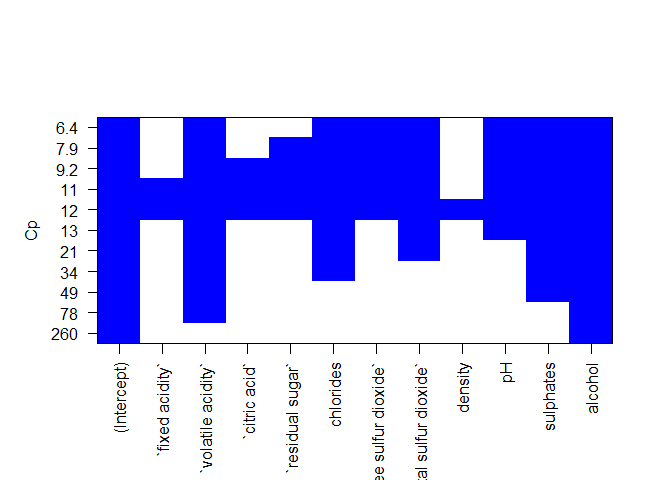
From the above plot we see a lowest Cp value around 6.4 comprising of predictor variable-
- Volatile acidity,chrolides,free sulphur dioxide,total sulphur dixide, pH,sulphates,alcohol.
- total number of predictor variables in the model -7
Model selection using 10 fold cross-validation
Training set MSE is generally an underestimate of the test MSE. This because when we fit a model to the training data using least squares we find the parameters for which the model minimizes the train MSE. So training error decreases as we increase more number of variables. So by picking a model with lowest train MSE, we may over fit the model. There are number of techniques for adjusting the training error for the model size. Few popular approaches are
- Akaike Information Criterion (AIC)
- Bayesian Information Criterion (BIC)
- adjusted R-squared
- Mallow’s Cp
- k-fold Cross validation
We have seen earlier to use the Cp criteria to find a best model. Now we’ll use 10-fold cross validation to pick the best model. The major advantage of using cross-validation is it doesn’t require σ2, variance of the irreducible error.
predict.regsubsets=function(object,newdata,id,...){
  form=as.formula(object$call[[2]])
  mat=model.matrix(form,newdata)
  coefi=coef(object,id=id)
  mat[,names(coefi)]%*%coefi
}
set.seed(2)
folds=sample(rep(1:10,length=nrow(wine_train)))
table(folds)
## folds
##   1   2   3   4   5   6   7   8   9  10
## 128 128 128 128 128 128 128 128 128 128
cv.errors=matrix(NA,10,11)
for(k in 1:10){
  best.fit=regsubsets(quality~.,data=wine_train[folds!=k,],nvmax=11,method="forward")
  for(i in 1:11){
    pred=predict(best.fit,wine_train[folds==k,],id=i)
    cv.errors[k,i]=mean( (wine_train$quality[folds==k]-pred)^2)
  }
}
rmse.cv=sqrt(apply(cv.errors,2,mean))
rmse.train=sqrt(best.fit$rss/(128*9))
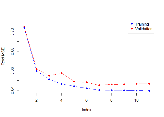
plot(rmse.cv,pch=19,type="b",col="red",ylab = "Root MSE",ylim=c(0.64,0.71))
points(rmse.train[-1],col="blue",pch=19,type="b")
legend("topright",legend=c("Training","Validation"),col=c("blue","red"),pch=19)
min(rmse.cv)
## [1] 0.6452647
As we expect, the training error goes down monotonically as the model gets bigger, but not so for the validation error. The cross-validated method results in a 7 variable model, similar to the mallow Cp approach. Lets check out the coefficients of the best model.
best.train=regsubsets(quality~.,data=wine_train,nvmax=11,method="forward")
id=which(rmse.cv==min(rmse.cv))
coef(best.train,id=id)
##            (Intercept)     `volatile acidity`              chlorides
##            4.394596302           -1.024064563           -1.988556904
##  `free sulfur dioxide` `total sulfur dioxide`                     pH
##            0.006914995           -0.003789943           -0.474617263
##              sulphates                alcohol
##            0.808678947            0.294192546
Next we test this model of the unused wine_test dataset comprising of 317 observations.
pred.test=predict.regsubsets(best.train,wine_test[],id=id)
test.error<-mean( (wine_test$quality-pred.test)^2)
test.error
## [1] 0.4535952
table(abs(wine_test$quality-round(pred.test)))
##
##   0   1   2
## 189 118  10
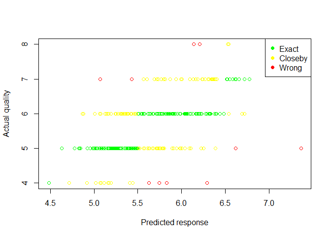
From the counts table we see our model has performed well as it accurately predict quality of 307/317 observations within 1 absolute quality difference, test MSE=0.4535
plot(pred.test,wine_test$quality,col="red",xlab="Predicted response",ylab="Actual quality")
points(pred.test[wine_test$quality==round(pred.test)],wine_test$quality[wine_test$quality==round(pred.test)],col="green")
points(pred.test[abs(wine_test$quality-round(pred.test))==1],wine_test$quality[abs(wine_test$quality-round(pred.test))==1],col="yellow")
legend("topright",legend=c("Exact","Closeby","Wrong"),col=c("green","yellow","red"),pch=19)
Inferences
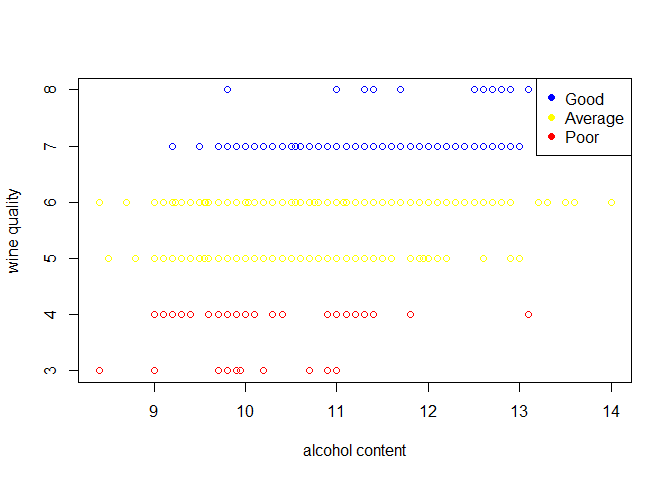
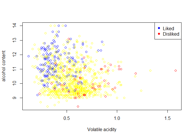
From the forward selection approach we see the variables alcohol and volatile acidity as the top two variables related to the wine quality. Also there is a medium correlation between the wine quality and alcohol content.
- The plot suggest that alcohol content ranging from 12%-15% are rated better.
- The wine with higher acidity have been rated poor quality, this emphasises the fact from studies which show wine having higher acidity generally have undesirable odour as the volatile components of wine-the chemicals responsible for the many fruity, earthy aromas-become more reluctant to diffuse. Such types of wine are disliked which is also seen from the plot that wine having higher volatile acidity are rated low.
plot(wine_train$alcohol,wine_train$quality,legend=c("high quality"),xlab = "alcohol content",ylab = "wine quality")
points(wine_train$alcohol[wine_train$quality>6],wine_train$quality[wine_train$quality>6],col="blue")
points(wine_train$alcohol[wine_train$quality<7&wine_train$quality>4],wine_train$quality[wine_train$quality<7&wine_train$quality>4],col="yellow")
points(wine_train$alcohol[wine_train$quality<5],wine_train$quality[wine_train$quality<5],col="red")
legend("topright",legend=c("Good","Average","Poor"),col=c("blue","yellow","red"),pch=19)
plot(wine_train$`volatile acidity`,wine_train$alcohol,xlab="Volatile acidity",ylab="alcohol content",col="yellow")
points(wine_train$`volatile acidity`[wine_train$quality>6],wine_train$alcohol[wine_train$quality>6],col="blue")
points(wine_train$`volatile acidity`[wine_train$quality<5],wine_train$alcohol[wine_train$quality<5],col="red")
legend("topright",legend=c("Liked","Disliked"),col=c("blue","red"),pch=19)

Leave a Comment