Case Study Iris Dataset-PART II
Welcome to part II of our case study. In this part we will be building popular classifier models such as
- KNN
- Multiclass Logistic Regression
- Linear Discriminant Analysis
K-Nearest Neighbour
KNN algorithm is one of the simplest classification algorithm and it is one of the most used learning algorithms. KNN is a non-parametric, lazy learning algorithm. Its purpose is to use a database in which the data points are separated into several classes to predict the classification of a new sample point. Its non-parametric , it means that it does not make any assumptions on the underlying data distribution. In other words, the model structure is determined from the data. KNN Algorithm is based on feature similarity: How closely out-of-sample features resemble our training set determines how we classify a given data point. The tuning parameters is “K”. We will use validation to determine it. As KNN use L2 distance measure between points its important to normalize our data points as different scales of variables changes the distance metric. Since in our case all the variables are similar scales we skip this step.
library(class)
knn.error=double(4)
knn.error2=double(4)
t=c(1,5,10,15,20)
ind=sample(1:120,90)
for(i in 1:5){
pred.knn.train=knn(train = trainset[ind,1:4], test = trainset[ind,1:4],cl = trainset[ind,]$Species, k=t[i])
pred.knn.test=knn(train = trainset[ind,1:4], test = testset[-ind,1:4],cl = trainset[ind,]$Species, k=t[i])
knn.error[i]=mean(trainset[ind,5]!=pred.knn.train)
knn.error2[i]=mean(testset[-ind,5]!=pred.knn.test)
}
matplot(t,cbind(knn.error,knn.error2),pch=19,col=c("red","blue"),type="b",ylab="Misclassification rate",xlab="K-no. of neighbours")
legend("topright",legend=c("Train","Validation"),pch=19,col=c("red","blue"))

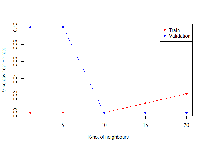
We see that a k=10 is an optimal choice for the tuning parameter.Note that for finding K we used an different validation set split from the training set to optimize it. After choice K, we can predict the classes for our unseen separted test set.
pred.knn.train=knn(train = trainset[,1:4], test = trainset[,1:4],cl = trainset$Species, k=10)
pred.knn.test=knn(train = trainset[,1:4], test = testset[,1:4],cl = trainset$Species, k=10)
accuracy.train[3]=mean(pred.knn.train==trainset$Species)
accuracy.validation[3]=mean(pred.knn.test==testset$Species)
confusionMatrix(pred.knn.test,testset$Species)
## Confusion Matrix and Statistics
##
##                  Reference
## Prediction        Iris-setosa Iris-versicolor Iris-virginica
##   Iris-setosa              10               0              0
##   Iris-versicolor           0               9              0
##   Iris-virginica            0               1             10
##
## Overall Statistics
##
##                Accuracy : 0.9667
##                  95% CI : (0.8278, 0.9992)
##     No Information Rate : 0.3333
##     P-Value [Acc > NIR] : 2.963e-13
##
##                   Kappa : 0.95
##  Mcnemar's Test P-Value : NA
##
## Statistics by Class:
##
##                      Class: Iris-setosa Class: Iris-versicolor
## Sensitivity                      1.0000                 0.9000
## Specificity                      1.0000                 1.0000
## Pos Pred Value                   1.0000                 1.0000
## Neg Pred Value                   1.0000                 0.9524
## Prevalence                       0.3333                 0.3333
## Detection Rate                   0.3333                 0.3000
## Detection Prevalence             0.3333                 0.3000
## Balanced Accuracy                1.0000                 0.9500
##                      Class: Iris-virginica
## Sensitivity                         1.0000
## Specificity                         0.9500
## Pos Pred Value                      0.9091
## Neg Pred Value                      1.0000
## Prevalence                          0.3333
## Detection Rate                      0.3333
## Detection Prevalence                0.3667
## Balanced Accuracy                   0.9750
cat("Training Accuracy:",accuracy.train[3],"\n" )
## Training Accuracy: 0.975
cat("Validation Accuracy:",accuracy.validation[3])
## Validation Accuracy: 0.9666667
We see an 97.5% accuracy on our training set and about 96.67% in our test set. Even though KNN is perceived as a lazy algorithm as it classifies a new data point based on the majority class in it neighbour, its a powerful algorithm does very well on many datasets.
Logistic Regression
In earlier projects, we have seen how a logistic regression can be used a classifier. We can extend the same idea to this classification problem. Our target variable is a factor variable with 3 levels, so for doing a multiclass logistic regression, we will use a one vs. all approach. In one vs. all approach, the target variable is encode into an indicator variable for each level and the newly created output vector is used to train a binary logistic regression. Similarly we fit models for other 2 classes as well. So in general for k level classifier, we build k binary logistic regression models.
#storing the class probabilities of train and test set
logit1 <- glm(I(trainset$Species=="Iris-setosa") ~ ., data=trainset, family='binomial')
logit2 <- glm(I(trainset$Species=="Iris-versicolor") ~ ., data=trainset, family='binomial')
logit3 <- glm(I(trainset$Species=="Iris-virginica") ~ ., data=trainset, family='binomial')
Here is a function which reurns the class probabilites.
classprobfn<-function(newdata){
  classprob=matrix(0,dim(newdata)[1],3)
  classprob[,1]=predict(logit1,newdata = newdata,type = "response")
  classprob[,2]=predict(logit2,newdata = newdata,type = "response")
  classprob[,3]=predict(logit3,newdata = newdata,type = "response")
  return(classprob)
}
Once the probabilities for each are calculated. We can classify a new data point to the class with highest probability.
classprob_train=classprobfn(trainset)
classprob_test=classprobfn(testset)
predictedclass_train<-max.col(classprob_train)
predictedclass_test<-max.col(classprob_test)
Since our logistic models uses indicator class response for modelling, the resulting classes are in factor levels og 1 to k. So we will encode our species variable into factor levels of 1,2,3 for easier comparison.
1-Iris-setosa 2-Iris-versicolor 3-Iris-virginica
species_encode = factor(iris$Species,
               levels = c('Iris-setosa', 'Iris-versicolor', 'Iris-virginica'),
               labels = c(1, 2, 3))
accuracy.train[4]=mean(predictedclass_train==species_encode[index])
accuracy.validation[4]=mean(predictedclass_test==species_encode[-index])
confusionMatrix(as.factor(predictedclass_test),species_encode[-index])
## Confusion Matrix and Statistics
##
##           Reference
## Prediction  1  2  3
##          1 10  0  0
##          2  0  8  0
##          3  0  2 10
##
## Overall Statistics
##
##                Accuracy : 0.9333
##                  95% CI : (0.7793, 0.9918)
##     No Information Rate : 0.3333
##     P-Value [Acc > NIR] : 8.747e-12
##
##                   Kappa : 0.9
##  Mcnemar's Test P-Value : NA
##
## Statistics by Class:
##
##                      Class: 1 Class: 2 Class: 3
## Sensitivity            1.0000   0.8000   1.0000
## Specificity            1.0000   1.0000   0.9000
## Pos Pred Value         1.0000   1.0000   0.8333
## Neg Pred Value         1.0000   0.9091   1.0000
## Prevalence             0.3333   0.3333   0.3333
## Detection Rate         0.3333   0.2667   0.3333
## Detection Prevalence   0.3333   0.2667   0.4000
## Balanced Accuracy      1.0000   0.9000   0.9500
cat("Training Accuracy:",accuracy.train[4],"\n" )
## Training Accuracy: 1
cat("Validation Accuracy:",accuracy.validation[4])
## Validation Accuracy: 0.9333333
Well our logistic model has performed very well on our training set yielding a error rate of 0%. From our earlier scatter plot we know a linear classifier can perform well as the boundary margin seems to be a linear plane in the 4 dimensions. We can find the class probabilities for our misclassified observation to get an understanding of difference in their probabilities.
classprob_test[which(predictedclass_test!=species_encode[-index]),]
##              [,1]      [,2] [,3]
## [1,] 2.220446e-16 0.8268286    1
## [2,] 2.220446e-16 0.6734220    1
species_encode[-index][which(predictedclass_test!=species_encode[-index])]
## [1] 2 2
## Levels: 1 2 3
The two misclassified observations belong to species Iris-versicolor. Their class probabilities are close to 1 but our binary model of species Iris-virginica seems to have probability 1.
Linear Dicriminant analysis
LDA makes some simplifying assumptions about your data:
- That your data is Gaussian, that each variable is shaped like a bell curve when plotted.
- That each attribute has the same variance, that values of each variable vary around the mean by the same amount on average.
With these assumptions, the LDA model estimates the mean and variance from your data for each class. LDA makes predictions by estimating the probability that a new set of inputs belongs to each class. The class that gets the highest probability is the output class and a prediction is made. The model uses Bayes Theorem to estimate the probabilities. This method was first proposed by Fisher and demonstrated using this Iris dataset which we are studying about.
fit.lda<-train(x = trainset[,1:4],y = trainset[,5], method = "lda",metric = "Accuracy")
pred.train.lda<-predict(object = fit.lda,newdata = trainset[,1:4])
pred.test.lda<-predict(object = fit.lda,newdata = testset[,1:4])
accuracy.train[5]=mean(pred.train.lda==trainset$Species)
accuracy.validation[5]=mean(pred.test.lda==testset$Species)
confusionMatrix(pred.test.lda,testset$Species)
## Confusion Matrix and Statistics
##
##                  Reference
## Prediction        Iris-setosa Iris-versicolor Iris-virginica
##   Iris-setosa              10               0              0
##   Iris-versicolor           0               9              0
##   Iris-virginica            0               1             10
##
## Overall Statistics
##
##                Accuracy : 0.9667
##                  95% CI : (0.8278, 0.9992)
##     No Information Rate : 0.3333
##     P-Value [Acc > NIR] : 2.963e-13
##
##                   Kappa : 0.95
##  Mcnemar's Test P-Value : NA
##
## Statistics by Class:
##
##                      Class: Iris-setosa Class: Iris-versicolor
## Sensitivity                      1.0000                 0.9000
## Specificity                      1.0000                 1.0000
## Pos Pred Value                   1.0000                 1.0000
## Neg Pred Value                   1.0000                 0.9524
## Prevalence                       0.3333                 0.3333
## Detection Rate                   0.3333                 0.3000
## Detection Prevalence             0.3333                 0.3000
## Balanced Accuracy                1.0000                 0.9500
##                      Class: Iris-virginica
## Sensitivity                         1.0000
## Specificity                         0.9500
## Pos Pred Value                      0.9091
## Neg Pred Value                      1.0000
## Prevalence                          0.3333
## Detection Rate                      0.3333
## Detection Prevalence                0.3667
## Balanced Accuracy                   0.9750
cat("Training Accuracy:",accuracy.train[5],"\n" )
## Training Accuracy: 0.9833333
cat("Validation Accuracy:",accuracy.validation[5])
## Validation Accuracy: 0.9666667
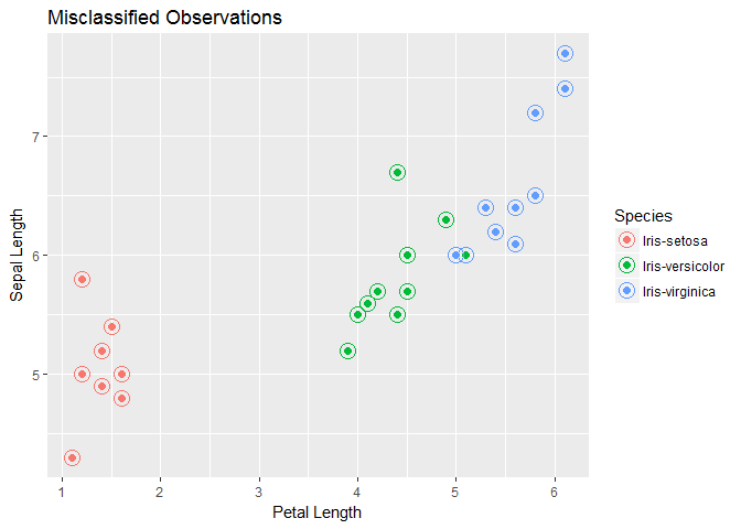
We see good results on both training and test sets. We get an accuracy of 98.33 on training set and 96.667 on test set. We see that there is only one misclassified observation. We will plot to see where the data point lies. The solid point in the plot represents the actual species class and circled data point is the predicted class.
misclass_lda<-ggplot(testset,aes(x=Petal.Length,y=Sepal.Length))+geom_point(aes(color=Species),size=2,pch=19)+geom_point(aes(color=pred.test.lda),pch=1,size=5)+xlab("Petal Length")+ylab("Sepal Length")+ggtitle("Misclassified Observations")
print(misclass_lda)

Summary
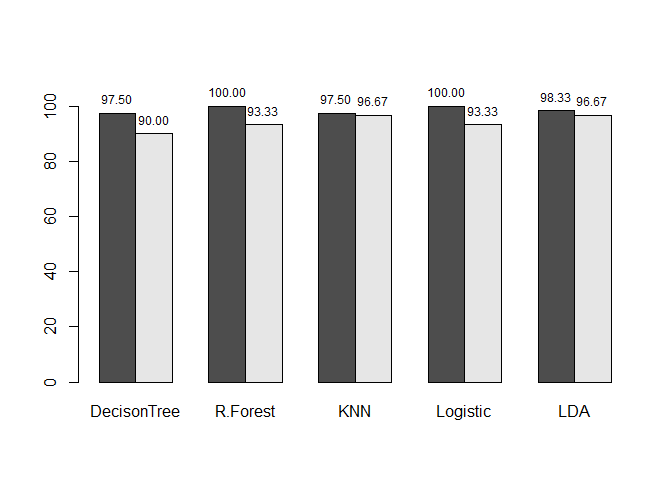
We have tried a few models on the Iris dataset which hopefully gives a broad overview of the variety of algorithms and models possible in R. As a final step we can summarize the results of our analysis by presenting the training and test set results for the models we employed. All the models have comparable results on our small dataset.
modelname<-c("DecisonTree","R.Forest","KNN","Logistic","LDA")
accuracy <- round(rbind(accuracy.train, accuracy.validation)*100,digits = 2)
mp <- barplot(accuracy, beside = TRUE,ylim = c(0, 110), names.arg = modelname)
text(mp, accuracy, labels = format(accuracy, 5),pos = 3, cex = .75)


Leave a Comment