Case Study Iris Dataset-PART I
This is perhaps the best known data set to be found in the classification literature. The aim is to classify iris flowers among three species (setosa, versicolor or virginica) from measurements of length and width of sepals and petals.
The iris data set contains 3 classes of 50 instances each, where each class refers to a type of iris plant. The central goal here is to design a model which makes good classifications for new data, in other words one which exhibits good generalization This is small dataset from Fisher’s paper published in 1936 and is often used for testing out machine learning algorithms and visualizations.
Our goal for this case study is to:
- Explore the Data
- Build and compare different classifiers
Overview of the Report
- Data exploration and Visualization
- Classification models
- Part I-Tree based models
- Decision trees
- Random Forest
- Part II- Other models
- Logistic Regression
- KNN
- Linear Discriminant Analysis
- Summarizing the models
Loading the required packages
library(caret)
library(readr)
library(rpart)
library(ggplot2)
library(tidyverse)
library(gridExtra)
library(RColorBrewer)
library(rattle)
library(knitr)
Loading the dataset
iris <- read_csv("C:/Users/subhash karthik/Desktop/blog content/iris/iris.data",
    col_names = FALSE)
iris<-data.frame(unclass(iris))
kable(head(iris),caption = "Iris dataset")
| X1 | X2 | X3 | X4 | X5 |
|---|---|---|---|---|
| 5.1 | 3.5 | 1.4 | 0.2 | Iris-setosa |
| 4.9 | 3.0 | 1.4 | 0.2 | Iris-setosa |
| 4.7 | 3.2 | 1.3 | 0.2 | Iris-setosa |
| 4.6 | 3.1 | 1.5 | 0.2 | Iris-setosa |
| 5.0 | 3.6 | 1.4 | 0.2 | Iris-setosa |
| 5.4 | 3.9 | 1.7 | 0.4 | Iris-setosa |
Here we see that the variable names are assigned by default. From the UCI repository we can find the details about the variables and lets rename the column names accordingly for further use.
colnames(iris)<-c("Sepal.Length","Sepal.Width","Petal.Length","Petal.Width","Species")
kable(head(iris),caption = "Iris dataset")
| Sepal.Length | Sepal.Width | Petal.Length | Petal.Width | Species |
|---|---|---|---|---|
| 5.1 | 3.5 | 1.4 | 0.2 | Iris-setosa |
| 4.9 | 3.0 | 1.4 | 0.2 | Iris-setosa |
| 4.7 | 3.2 | 1.3 | 0.2 | Iris-setosa |
| 4.6 | 3.1 | 1.5 | 0.2 | Iris-setosa |
| 5.0 | 3.6 | 1.4 | 0.2 | Iris-setosa |
| 5.4 | 3.9 | 1.7 | 0.4 | Iris-setosa |
set.seed(99)
The dataset is split into train and validation set. The validation set will be unseen by the ML model and we’ll also explore the data using only the training set so that no form of training is done with our validation set.
# We use the dataset to create a partition (80% training 20% testing)
index <- createDataPartition(iris$Species, p=0.80, list=FALSE)
# select 20% of the data for testing
testset <- iris[-index,]
# select 80% of data to train the models
trainset <- iris[index,]
Explore the Data
Since we are dealing here with a clean and small dataset we are able to avoid the step of Cleaning the data which typically consumes a majority of the data scientists’ time.
We explore the data to:
- Understand the data
- Summarize the data
- Understand relationships between variables
- Think about the types of models to fit the data
Summarizing the data
We will see the dimension of our dataset and structure of it and finally the each variable summary statistics.
dim(trainset)
## [1] 120 5
str(trainset)# structure
## 'data.frame':    120 obs. of  5 variables:
##  $ Sepal.Length: num  5.1 4.7 4.6 5 5.4 4.6 5 4.4 4.9 5.4 ...
##  $ Sepal.Width : num  3.5 3.2 3.1 3.6 3.9 3.4 3.4 2.9 3.1 3.7 ...
##  $ Petal.Length: num  1.4 1.3 1.5 1.4 1.7 1.4 1.5 1.4 1.5 1.5 ...
##  $ Petal.Width : num  0.2 0.2 0.2 0.2 0.4 0.3 0.2 0.2 0.1 0.2 ...
##  $ Species     : Factor w/ 3 levels "Iris-setosa",..: 1 1 1 1 1 1 1 1 1 1 ...
summary(trainset)# variable summary
##   Sepal.Length    Sepal.Width     Petal.Length    Petal.Width
##  Min.   :4.400   Min.   :2.000   Min.   :1.000   Min.   :0.100
##  1st Qu.:5.100   1st Qu.:2.800   1st Qu.:1.500   1st Qu.:0.300
##  Median :5.800   Median :3.000   Median :4.300   Median :1.300
##  Mean   :5.848   Mean   :3.071   Mean   :3.747   Mean   :1.201
##  3rd Qu.:6.425   3rd Qu.:3.300   3rd Qu.:5.100   3rd Qu.:1.800
##  Max.   :7.900   Max.   :4.400   Max.   :6.900   Max.   :2.500
##             Species
##  Iris-setosa    :40
##  Iris-versicolor:40
##  Iris-virginica :40
##
##
##
levels(trainset$Species)
## [1] "Iris-setosa" "Iris-versicolor" "Iris-virginica"
Verifies the fact that there are three types of species i.e. our target Species is a factor variable with 3 levels. Also from our summary statistics we see the class distribution is equal.
Data visualization
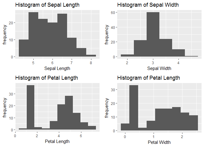
Using ggplot library we will visaulize the distribution of each predictor variable and explore it.
hist_sepl<-ggplot(trainset,aes(x=Sepal.Length))+geom_histogram(binwidth = 0.5)+xlab("Sepal Length")+ylab("frequency")+ggtitle("Histogram of Sepal Length")

hist_sepw<-ggplot(trainset,aes(x=Sepal.Width))+geom_histogram(binwidth = 0.5)+xlab("Sepal Width")+ylab("frequency")+ggtitle("Histogram of Sepal Width")

hist_petl<-ggplot(trainset,aes(x=Petal.Length))+geom_histogram(binwidth = 0.7)+xlab("Petal Length")+ylab("frequency")+ggtitle("Histogram of Petal Length")

hist_petw<-ggplot(trainset,aes(x=Petal.Width))+geom_histogram(binwidth = 0.3)+xlab("Petal Width")+ylab("frequency")+ggtitle("Histogram of Petal Length")
grid.arrange(hist_sepl,hist_sepw,hist_petl,hist_petw,nrow=2)
We will observe the relationship between Sepal dimensions with each Species and similarly with petal dimensions also.
scatter_sepal<-ggplot(trainset,aes(x=Sepal.Length,y=Sepal.Width,color=Species))+geom_point(size=2)+ggtitle("Sepal Length vs Sepal Width")
scatter_petal<-ggplot(trainset,aes(x=Petal.Length,y=Petal.Width,color=Species))+geom_point(size=2)+ggtitle("Petal Length vs Petal Width")
grid.arrange(scatter_sepal,scatter_petal,nrow=2)
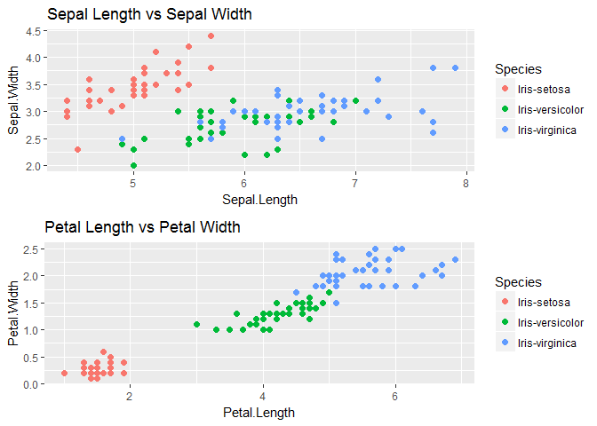
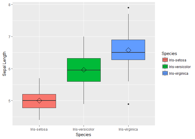
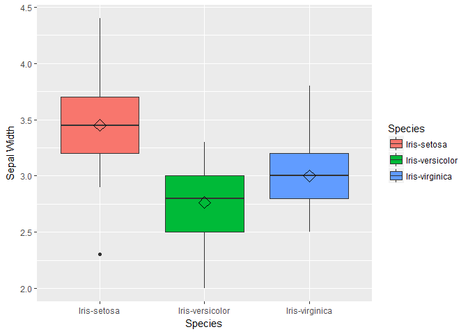
We see that One class-Iris-Setosa is linearly separable from the other 2; the latter are NOT linearly separable from each other. Next we will visualize variable distribution using box plots for each species type.
box1 <- ggplot(data=trainset, aes(x=Species, y=Sepal.Length))+  geom_boxplot(aes(fill=Species)) + ylab("Sepal Length") + stat_summary(fun.y=mean, geom="point", shape=5, size=4)
box2 <- ggplot(data=trainset, aes(x=Species, y=Sepal.Width))+  geom_boxplot(aes(fill=Species)) + ylab("Sepal Width")  + stat_summary(fun.y=mean, geom="point", shape=5, size=4)
box3 <- ggplot(data=trainset, aes(x=Species, y=Petal.Length))+  geom_boxplot(aes(fill=Species)) + ylab("Petal Length") + stat_summary(fun.y=mean, geom="point", shape=5, size=4)
box4 <- ggplot(data=trainset, aes(x=Species, y=Petal.Width))+  geom_boxplot(aes(fill=Species)) + ylab("Petal Width") +stat_summary(fun.y=mean, geom="point", shape=5, size=4)
box1;box2;box3;box;
## function (which = "plot", lty = "solid", ...)
## {
##     which <- pmatch(which[1L], c("plot", "figure", "inner", "outer"))
##     .External.graphics(C_box, which = which, lty = lty, ...)
##     invisible()
## }
## <bytecode: 0x000000000ffb6360>
## <environment: namespace:graphics>
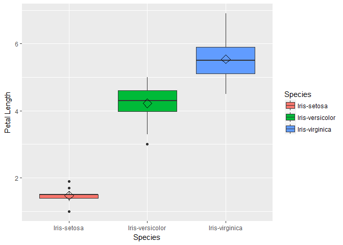
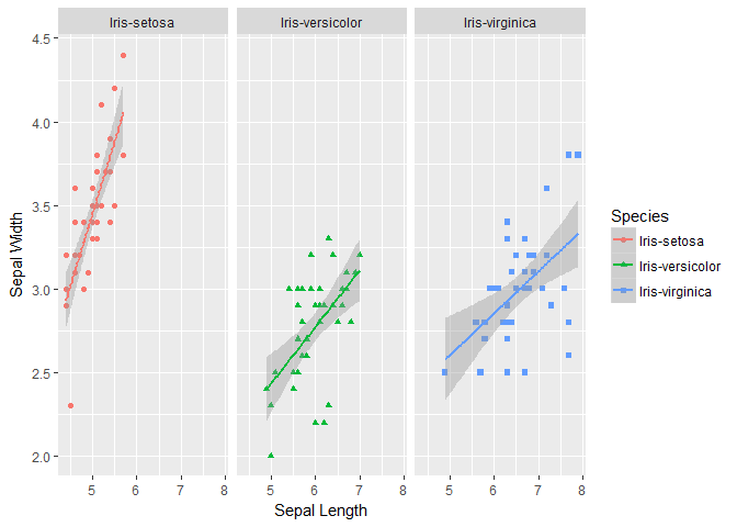
For the bar plots of Petal length we see that the mean and distribution for each class are well separated. We can conclude petal length may be a important variable in our models. Also note that the distribution of sepal length and petal width are similar, so lets plot these two variable to check how linearly they are related.
sepal_petal <- ggplot(data=trainset, aes(Sepal.Length, y=Sepal.Width, color=Species))+
    geom_point(aes(shape=Species), size=1.5)+geom_smooth(method="lm")+xlab("Sepal Length") + ylab("Sepal Width") +facet_grid(. ~ Species) # Along rows
print(sepal_petal)
Building ML Models
The training and test set accuracy are stored for later comparison purposes.
accuracy.train=double(5)
accuracy.validation=double(5)
Tree based methods
Decision Trees
A decision tree is a structure that includes a root node, branches, and leaf nodes. Each internal node denotes a test on an attribute, each branch denotes the outcome of a test, and each leaf node holds a class label. The topmost node in the tree is the root node. In decision analysis, a decision tree can be used to visually and explicitly represent decisions and decision making. Advantages of CART * Simple to understand, interpret, visualize. * Decision trees implicitly perform variable screening or feature selection. * Can handle both numerical and categorical data. Can also handle multi-output problems. * Nonlinear relationships between parameters do not affect tree performance.
We will fit a simple rpart algorithm to grow a tree on our training dataset and use it to predict on the unseen test set.
fit.rpart <- rpart(Species ~., data = trainset)
fancyRpartPlot(fit.rpart)
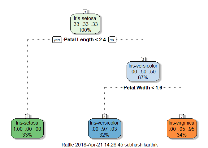
The grow tree is very simple in structure and easily interpretable. Remember we had a hunch that petal length is important feature see that our decision tree(DT) uses it as a decision maker to create two nodes of which one is a leaf node which is purer too, containing only setosa class as DT’s split the variable space into boxes for creating new nodes. The two leaf nodes are almost pure just containing a few other class observations. Next we will use this DT to find the classification accuracy on our training and test datasets.
pred.train.rpart<-predict(fit.rpart,newdata = trainset[,1:4],type="class")
accuracy.train[1]=mean(pred.train.rpart==trainset$Species)
pred.test.rpart<-predict(fit.rpart,newdata = testset[,1:4],type="class")
accuracy.validation[1]=mean(pred.test.rpart==testset$Species)
confusionMatrix(pred.test.rpart,testset$Species)
## Confusion Matrix and Statistics
##
##                  Reference
## Prediction        Iris-setosa Iris-versicolor Iris-virginica
##   Iris-setosa              10               0              0
##   Iris-versicolor           0              10              3
##   Iris-virginica            0               0              7
##
## Overall Statistics
##
##                Accuracy : 0.9
##                  95% CI : (0.7347, 0.9789)
##     No Information Rate : 0.3333
##     P-Value [Acc > NIR] : 1.665e-10
##
##                   Kappa : 0.85
##  Mcnemar's Test P-Value : NA
##
## Statistics by Class:
##
##                      Class: Iris-setosa Class: Iris-versicolor
## Sensitivity                      1.0000                 1.0000
## Specificity                      1.0000                 0.8500
## Pos Pred Value                   1.0000                 0.7692
## Neg Pred Value                   1.0000                 1.0000
## Prevalence                       0.3333                 0.3333
## Detection Rate                   0.3333                 0.3333
## Detection Prevalence             0.3333                 0.4333
## Balanced Accuracy                1.0000                 0.9250
##                      Class: Iris-virginica
## Sensitivity                         0.7000
## Specificity                         1.0000
## Pos Pred Value                      1.0000
## Neg Pred Value                      0.8696
## Prevalence                          0.3333
## Detection Rate                      0.2333
## Detection Prevalence                0.2333
## Balanced Accuracy                   0.8500
cat("Training Accuracy:",accuracy.train[1],"\n" )
## Training Accuracy: 0.975
cat("Validation Accuracy:",accuracy.validation[1])
## Validation Accuracy: 0.9
We see an 97.5% accuracy on our training set and about 90% in our test set. See that one our DT leaf node is purer so the test set recall and precision of setosa class is equal to 1, so our wrongly classified ones belong to other two class.
Random Forest
These methods grow multiple trees which are then combined to yield a single consensus prediction. Combining a large number of trees can often result in dramatic improvements in prediction accuracy, at the expense of some loss interpretation. Here in random forest, when building these decision trees, each time a split in a tree is considered, a random selection of m predictors is chosen as split candidates from the full set of p predictors. The split is allowed to use only one of those m predictors. The tuning parameter is adjusted by “mtry” usually for a classification mtry is set as sqrt(p). Since in our problem p is 4(a very small number), so we will continue with the default mtry
library(randomForest)
fit.rf<-randomForest(Species~.,data=trainset)
fit.rf
##
## Call:
##  randomForest(formula = Species ~ ., data = trainset)
##                Type of random forest: classification
##                      Number of trees: 500
## No. of variables tried at each split: 2
##
##         OOB estimate of  error rate: 3.33%
## Confusion matrix:
##                 Iris-setosa Iris-versicolor Iris-virginica class.error
## Iris-setosa              40               0              0        0.00
## Iris-versicolor           0              38              2        0.05
## Iris-virginica            0               2             38        0.05
pred.train.rf<-predict(fit.rf,newdata = trainset[,1:4],type="class")
accuracy.train[2]=mean(pred.train.rf==trainset$Species)
pred.test.rf<-predict(fit.rf,newdata = testset[,1:4],type="class")
accuracy.validation[2]=mean(pred.test.rf==testset$Species)
confusionMatrix(pred.test.rf,testset$Species)
## Confusion Matrix and Statistics
##
##                  Reference
## Prediction        Iris-setosa Iris-versicolor Iris-virginica
##   Iris-setosa              10               0              0
##   Iris-versicolor           0               9              1
##   Iris-virginica            0               1              9
##
## Overall Statistics
##
##                Accuracy : 0.9333
##                  95% CI : (0.7793, 0.9918)
##     No Information Rate : 0.3333
##     P-Value [Acc > NIR] : 8.747e-12
##
##                   Kappa : 0.9
##  Mcnemar's Test P-Value : NA
##
## Statistics by Class:
##
##                      Class: Iris-setosa Class: Iris-versicolor
## Sensitivity                      1.0000                 0.9000
## Specificity                      1.0000                 0.9500
## Pos Pred Value                   1.0000                 0.9000
## Neg Pred Value                   1.0000                 0.9500
## Prevalence                       0.3333                 0.3333
## Detection Rate                   0.3333                 0.3000
## Detection Prevalence             0.3333                 0.3333
## Balanced Accuracy                1.0000                 0.9250
##                      Class: Iris-virginica
## Sensitivity                         0.9000
## Specificity                         0.9500
## Pos Pred Value                      0.9000
## Neg Pred Value                      0.9500
## Prevalence                          0.3333
## Detection Rate                      0.3000
## Detection Prevalence                0.3333
## Balanced Accuracy                   0.9250
From the model summary we see that random forest has used No. of variables tried at each split: 2 i.e. mtry =2 and number of trees grown is 500. One can show that on average, each bagged tree makes use of around two-thirds of the observations. The remaining one-third of the observations not used to fit a given bagged tree are referred to as the out-of-bag (OOB) observations. We can predict the response for the ith observation using each of the trees in which that observation was OOB. This total error is denoted as OOB error estimate which is calculated to be 3.33%.
cat("Training Accuracy:",accuracy.train[2],"\n" )
## Training Accuracy: 1
cat("Validation Accuracy:",accuracy.validation[2])
## Validation Accuracy: 0.9333333
Our OOB error estimate was 3.33% but overall prediction from all bags is having an error of zero ie. our Random forest model has classified correctly all observations from our training set. We get an accuracy of 93.333% on our test dataset which is an improvement from our decision tree model
In the subsequent post/article we will build other powerful classifier such as LDA, Logistic regression and KNN. Stay tuned

Leave a Comment