Central Limit Theorem

The central limit theorem states that if you have a population with mean μ and standard deviation σ and take sufficiently large random samples from the population, then the distribution of the sample means will be approximately normally distributed. This will hold true regardless of whether the source population is normal or skewed, provided the sample size is sufficiently large(usually n > 30).

$$\bar X\rightarrow N(\mu,\frac{\sigma}{n}),n\rightarrow\infty$$

According to the central limit theorem, the mean of a sampling distribution of means is an unbiased estimator of the population mean
$\mu_{\bar X}=\mu$

The standard deviation of resulting sampling distribution is given by
$\sigma_{\bar X}=\frac{\sigma}{\sqrt{n}}$

Example: We will use CLT to estimate the mean of student age who have participated in a survey.

Lets first see how the population data is distributed.

age<-StudentSurvey$age
hist(age,xlab = "age",ylab = "frequency",main="Histogram of students age")

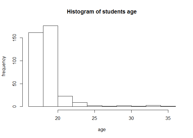
We can clearly see that the distribution is positively skewed.Lets calculate the mean and standard deviation of the distribution.

cat("Mean ",mean(age),"\n")

## Mean  19.25594

cat("Standard deviation ",sd(age),"\n")

## Standard deviation  2.269055

In this case we know we know the true population parameters, but often we dont have the population data. In such cases CLT provides an easier way to estimate the true population parameters.Now we use the power, CLT has provided to estimate them using different sampling size n=5,15,25,35.We will draw 1000 samples of size n from the data and estimate mean and SD.

samplefn<-function(age,size){
xbar <-rep(NA, 1000)
for (i in 1:1000)
{x <-sample(age, size =size)
 xbar[i] <-  mean(x)}
return(xbar)
}  

Case 1: Sample Size n=1

n=5
xbar<-samplefn(age,n)
# Graph the histogram of 1,000 sample means.
hist(xbar,xlab = "sample means",ylab = "frequency",main="Sampling distribution(n=5)")

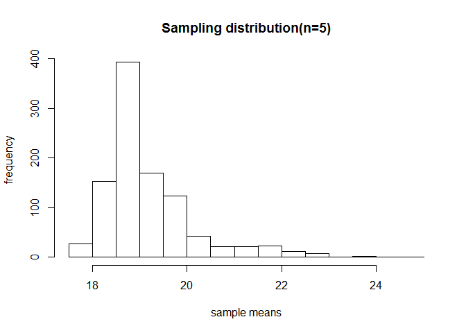
# Calculate the mean and sd of the sampling distribution.
cat("True mean",mean(age),"Estimated mean",mean(xbar),"\n")

## True mean 19.25594 Estimated mean 19.2248

cat("True SD",sd(age),"Estimated SD",sd(xbar)*sqrt(n),"\n")

## True SD 2.269055 Estimated SD 2.184238

Case 2: Sample size n=15

n=15
xbar<-samplefn(age,n)
# Graph the histogram of 1,000 sample means.
hist(xbar,xlab = "sample means",ylab = "frequency",main="Sampling distribution(n=15)")

# Calculate the mean and sd of the sampling distribution.
cat("True mean",mean(age),"Estimated mean",mean(xbar),"\n")

## True mean 19.25594 Estimated mean 19.25747

cat("True SD",sd(age),"Estimated SD",sd(xbar)*sqrt(n),"\n")

## True SD 2.269055 Estimated SD 2.212727

Case 3: Sample size n=25

n=25
xbar<-samplefn(age,n)
# Graph the histogram of 1,000 sample means.
hist(xbar,xlab = "sample means",ylab = "frequency",main="Sampling distribution(n=25)")

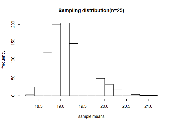
# Calculate the mean and sd of the sampling distribution.
cat("True mean",mean(age),"Estimated mean",mean(xbar),"\n")

## True mean 19.25594 Estimated mean 19.24584

cat("True SD",sd(age),"Estimated SD",sd(xbar)*sqrt(n),"\n")

## True SD 2.269055 Estimated SD 2.159808

Case 4: Sample size n=35

n=35
xbar<-samplefn(age,n)
# Graph the histogram of 1,000 sample means.
hist(xbar,xlab = "sample means",ylab = "frequency",main="Sampling distribution(n=35)")

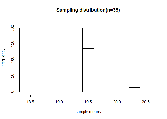
# Calculate the mean and sd of the sampling distribution.
cat("True mean",mean(age),"Estimated mean",mean(xbar),"\n")

## True mean 19.25594 Estimated mean 19.25689

cat("True SD",sd(age),"Estimated SD",sd(xbar)*sqrt(n),"\n")

## True SD 2.269055 Estimated SD 2.177265

From the above plots we see that as we increase the sample size, the sampling distribution becomes more normal and it becomes a better unbiased estimator of true population parameters.This simple example shows us how valuable CLT is to statistians making our inferences better from sample rather than conducting census which is a tedious process.